In 1963 Edward Lorenz published his famous set of coupled nonlinear
first-order ordinary differential equations; they are relatively simple,
but the resulting behavior is wonderfully complex. The equations are:
dx/dt = s(y-x)
dy/dt = rx-y-xz
dz/dt = xy – bz
with suggested parameters s=10, r=28, and b=8/3. The solution executes
a trajectory, plotted in three dimensions, that winds around and around,
neither predictable nor random, occupying a region known as its attractor.
With lots of computing power you can approximate the equations numerically,
and many handsome plots can be found on the web. However, it’s rather
easy to implement these equations in an analog electronic circuit, with
just 3 op-amps (each does both an integration and a sum) and two analog
multipliers (to form the products xy and xz).
The Circuit
Here’s the circuit:

It’s not hard to understand: the op-amps are wired as integrators, with
the various terms that make up each derivative summed at the inputs. The
resistor values are scaled to 1 megohm, thus for example R3 weights the
variable x with a factor of 28 (1M/35.7k); this is combined with -y and
-xz, each with unit weight. (note: the equations on the diagram are
normalized to 0.1V, hence the multiplier scale factor of 100.)
The Output
The circuit just sits there and produces three voltages x(t), y(t), and z(t);
if you hook x and z into a `scope, you get a pattern like this…

…the characteristic “owl’s face” of the Lorenz attractor. The curve
plays out in time, sometimes appearing to hesitate as it scales the
boundary and decides which basin to drop back into. The value of C, the
three integrator capacitors, sets the time scale: at 0.47uF it does a
leisurely wander; at 0.1uF it winds around like someone on a mission; and
at 0.002uF it is fiercely busy solving its equations and delighting its
audience.
http://www.malinc.se/m/Lorenz.php
http://physics.ucsc.edu/~drip/programs/lorenz/
Now whatever could that be used for in “NOISE”?
There are three Lorenz equations that comprise the Lorenz Attractor, each of which can be though of as the x, y, or z component of a given three dimensional location in space:
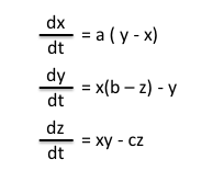
Each of these equations can be read as the ‘change in x,y, or z with respect to time’. Thus, each equation is used to calculate how much a given point is changed relative to the previous point, the change dependent upon the elapsed time.
The values a, b, c in the Lorenz equations are constants (for the Lorenz Attractor, a = 10, b = 28, and c = 8/3). These constants, as well as the above equations, can be altered to generate different results. For instance, a value of a = 1 results in a spiral with a single attractor (converging on this attractor), or a value of c = 20 results in a similar pattern given by c = 28, but with more compact orbits. Alternatively, other mathematical equations result in other types of attractors, such as the Henon Map or the Rossler Attractor.