Eye made this midi utility project ages ago because needed specific Arpeggiator function/pattern….
works as VSTi insert….
Writes MIDI into sequencer from external controller

Eye made this midi utility project ages ago because needed specific Arpeggiator function/pattern….
works as VSTi insert….
Writes MIDI into sequencer from external controller
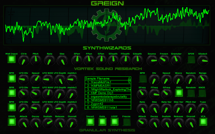
Revised/Rebuilt GREIGN Ganular Synthesis FX VST… for GREIGN STORM VSTi…
Bank of 8 source waves that can be selected or random play all of them… at random file read positions on BPM sync or using static injector for random voltage that selects any file… this is in super experimental mode now… alpha testing
My recent experiment for the past 3 days
so…. did some brainstorming…
plus R&D on granular synthesis
mentally dissected “clouds” module
circuit flowchart
thus with much experimentation plus overcoming obstacles via trial & error method
this is the result
Eye wanted something that created Ganular “clouds” in realtime
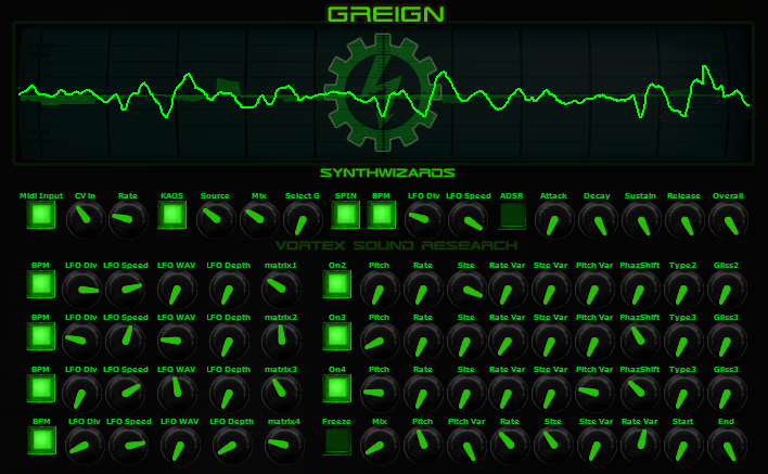
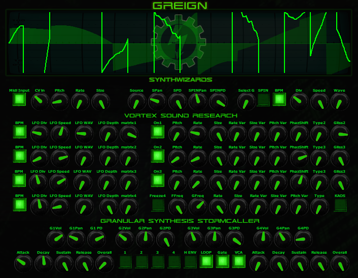
GREIGN has 4x Granulators
utilizing & expanding/evolving methods that Eye devised when redesigning NekroFile
This is used in conjunction with KaodMidiFire “KMF” generating psuedo randomized MIDI
creating 4 banks of clouds from audio input
some extreme modulating capabilities with 4 LFOs
plus added ability shuffling through the clouds
using BPM Sync LFO div from 16measures to 1/16th range
plus wide range free running LFO
Time for Recording
GREIGN graduates from ALPHA
Major Revision1: added pan/autopan for each cloud… added External MIDI control of ADSR for each cloud with separate Volume controls… Added secondary ADSR for modulating clouds….drastic buffer Size increase… added global pitch rate & size controls for clouds
|
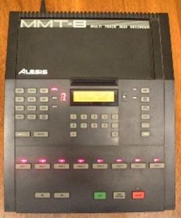
| 16x memory expansion mod
This modification expands the sequence memory by 16 times the original memory. Just like the original memory, the expanded memory retains all your sequences and songs even when you switch it off. The only limitation of this memory expansion is that each of the 16 memory spaces are isolated from each other, so you can’t use part 5 from memory space 1 and part 6 from memory space 2 and put them into a song in memory space 3. You create your songs in one memory and fill it, then switch to the next memory bank and start there etc.
There were 2 basic variants of the MMT8—the grey cased version, and the black cased version. Make sure you download the guide for your particular version—the guides are slightly different for the 2 variants |
| Download the Grey MMT8 memory expansion guide here |
| Download the Black MMT8 memory expansion guide here |
| DC/Batteries power mod
This modification enables you to run the MMT8 from a DC 12V power pack, which is much more common and available than the AC 9V power pack that normally powers the MMT8. It also then enables you to run it off rechargeable AA batteries! NOTE – this mod is only for the grey cased MMT8s – it won’t work for the black cased ones. |
| Download the DC/Batteries power mod here |
| To download the guides, right click on the below links and select “save target as” |
| To download the guide, right click on the link and select “save target as” |
Clouds continuously records the incoming audio into a short amount of sample memory. While recording time can reach up to 8s by reducing the audio quality setting, you ought to feel very guilty every time you think of this as “tape” – think of it as a space, a room. Using this recorded audio data, the module synthesizes a sonic texture by playing back short (overlapping) segments of audio (also known as “grains”) extracted from it.
Clouds allows you to control:
The module plays grains continuously, at a rate determined by the DENSITY and SIZE settings. A trigger input is also present, to explicitly instruct the module to start the playback of a new grain. The maximum number of concurrent grains is quite large – between 40 and 60. This specificity brings Clouds closer to the roots of granular synthesis, and allows the synthesis of varied textures even from basic waveforms – there’s indeed many more dimensions to granular synthesis than keeping a playback pointer moving through a SD-card sample!
It is possible, at any time, to FREEZE the audio buffer from which the grains are taken – In this case, the incoming audio is no longer recorded. Somehow, Clouds is the exact opposite of a sampler: by default, the module always samples the audio it receives, except when it is in the frozen state.
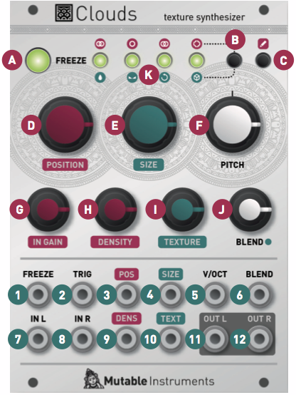
A. FREEZE button. This latching button stops the recording of incoming audio. Granularization is now performed on the last few seconds of audio kept in memory in the module.
B. Blending parameter/Audio quality button. Selects which of the blending parameters is controlled by the BLEND knob and CV input, or selects one of the four audio quality settings.
C. Load/Save button. See the “Advanced topics” section.
D. Grain POSITION. Selects from which part of the recording buffer the audio grains are played. Turn the knob clockwise to travel back in time.
E. F. Grain SIZE and PITCH (transposition). At 12 o’clock, the buffer is played at its original frequency.
G. Audio INPUT GAIN, from -18dB to +6dB.
H. Grain DENSITY. At 12 o’clock, no grains are generated. Turn clockwise and grains will be sown randomly, counter-clockwise and they will be played at a constant rate. The further you turn, the higher the overlap between grains.
I. Grain TEXTURE. Morphs through various shapes of grain envelopes: square (boxcar), triangle, and then Hann window. Past 2 o’clock, activates a diffuser which smears transients.
J. BLEND knob. This multi-function knob is described in the Blending parameters section.
K. Indicator LEDs. They work as an input vu-meter. When FREEZE is active, they monitor the output level. Soft-clipping occurs when the last LED is on. They can also indicate the quality setting (red), the function assigned to the BLEND knob (green), or the value of the four blending parameters (multicolor).
All CV inputs are calibrated for a range of +/- 5V. Voltages outside of this range are tolerated, but will be clamped.
1. FREEZE gate input. When the input gate signal is high, stops the recording of incoming audio, just as latching the FREEZE button would do.
2. TRIGGER input. Generates a single grain. By moving the grain DENSITY to 12 o’clock, and sending a trigger to this input, Clouds can be controlled like a micro-sample player. An LFO or clock divider (or even a pressure plate) can thus be used to sow grains at the rate of your choice.
3. 4. Grain POSITION and SIZE CV inputs.
5. Grain transposition (PITCH) CV input, with V/Oct response.
6. BLEND CV input. This CV input can control one of the following functions depending on the active blending parameter: dry/wet balance, grain stereo spread, feedback amount and reverb amount.
7. 8. Stereo audio input. When no patch cable is inserted in the right channel input, this input will receive the signal from the left channel.
9. 10. Grain DENSITY and TEXTURE CV inputs.
11. 12. Stereo audio output.
The BLEND knob can control one of these four settings:
To select which parameter is controlled by the BLEND knob and the BLEND CV input, press the Blend parameter/Audio quality button. The current parameter is temporarily indicated by a green LED.
When turning the BLEND knob, the color of the four status LEDs temporarily shows the value of the four blending parameters (from black when the parameter is set to its minimum value to green, yellow and then red for the maximum value).
It could happen that the position of the knob does not match the value of the parameter – the curse of multi-function knobs! If this is the case, turning the BLEND knob clockwise (resp. counterclockwise) causes a small increase (resp. decrease) in the value of the parameter, and turning it further causes larger changes, until the value progressively catches up with the knob’s position.
There are a few things worth knowing about these settings:
Hold the Blend parameter/Audio quality button for one second, then press it repeatedly to choose a recording quality. The current quality setting is indicated by a red LED.
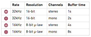
Note that Clouds’ 8-bit is a lovely flavour of 8-bit: µ-law companding. It sounds like a Cassette, or a Fairlight – less hiss, more distortion.
Up to 4 frozen audio buffers can be saved and reloaded. Along with the audio data itself, the quality settings and the processing mode are saved with it. To save the recording buffer in permanent memory:
To load a recording buffer from permanent memory:
If you press the Load/Save button by mistake, do not press any button for a few seconds and the module will return to its normal state.
A grain of sound is a brief acoustical event, with a duration near the treshold of human perception (usually between 10 and 60 milliseconds). The idea behind granular synthesis is the creation of complex soundscapes by combining thousands of grains of sound over time. In granular synthesis, a grain of sound is considered as a building block for the creation of more complex sonic events. An example of a grain of sound is shown in Figure 1.

|
The idea of having sound grains was proposed by the British physicist Dennis Gabor in 1947. Gabor suggested the idea of a quantum of sound, as a perceptual indivisible unit of information. All macro-level phenomena are based on the sound quantum.
Granular synthesis was first suggested as a computer music technique for producing complex sounds by Iannis Xenakis and Curtis Roads.
Granular synthesis is based on the production of a high density of small acoustic events called grains that are typically in the range of 10-60 ms.
To enable smooth transitions between grains, each grain has an amplitude envelope. In Gabor’s original conception, the amplitude envelope is a bell shaped curve generated by the Gaussian method:
 |
(1) |
Figure 2 shows different kinds of amplitude envelopes. Notice that, for computational purposes, simple envelopes such as triangular can be used.
When the envelope is applied to the grain, the effect shown in Figure 3 is produced.

|

|
The control parameters of a granular synthesizer are the following:
Typical grain densities range from several hundred to several thousand grains per second.

|

|

|

|
When organized over time, grains can be placed in a synchronous or asynchronous way.
In synchronous granular synthesis, grains are placed at equally spaced positions. This creates a periodicity which provides a sensation of frequency. For example, if grains are placed every 10 ms, a 100 Hz frequency will be heard.
A technique designed for the synthesis of tones with one or more resonances, i.e. this technique is suitable for imitating natural instruments and voices. All the grains are regularly placed over time.
In asynchronous granular synthesis, grains are scattered randomly over a user-determined duration and with user-determined density and frequency content (depending on the waveform used in the grains).
Granular synthesis can be implemented generating small sound events and placing them over time as if in a score. Lots of parameters are involved. Their choice and organisation is what makes granular synthesis more or less interesting.
In synchronous granular synthesis, it is possible to create time stretching effects by repeating the grains is a longer (or shorter) amount of time, without varying their distance.
In synchronous granular synthesis, it is possible to create pitch shifting effects by changing the space between the grains.
Granular synthesis has been extensively used in computer music for its high flexibility in manipulating sounds. Composers such as Xenakis, to cite just a few, has been using granular synthesis in their creative work.
Recently granular synthesis has also been used in computer games, to generate interactive soundscapes.
With regard to sampling (3.3) you learned how to change the speed of an existing sound in an array, but this also resulted in a change of pitch. One way to decouple these parameters, is by using granular synthesis. The idea of granular synthesis is that a sound is sampled at the original speed, but it is played at a different speed from each sample point.
You have an “indicator” that moves across the array at normal speed:
patches/3-7-1-1-granular-theory1.pd

Only at certain intervals do we get information about the indicator’s present position; when this information is received, the array is played back from that point, albeit at a different speed.
To understand this better, let’s say this is the normal playback speed:

…and this is a speed that is ‘too fast’:

…then granular synthesis does this:

Though playback is ‘too fast’ (or ‘too slow’), it always begins at a point that corresponds to the initial speed. These individual chunks are called “grains”; their size is referred to either as “grain size” or “window size”. These “grains” are so tiny and used in such large quantities, that they are not heard individually, but rather as a continuous whole. That’s the magic behind granular synthesis.
Every individual “grain” is played back like this:

After a grain is played, there is a jump to the next position; this position is taken from the current position of the “main indicator”. There is a special object to accomplish this: “samphold~”. It works like “spigot”, only on the signal level. Both the left and right inlets receive a signal. When there is descending step in the right inlet, “samphold~” immediately sends the sample currently in the left inlet and repeats this until the value in the right inlet is lower than the preceding one. This somewhat strange setting makes sense if the right input is a “phasor~”. It receives only once – right at the end of a period – a descending step. A grain could be read out this way and the offset could be added to the end of it:
patches/3-7-1-1-granular-theory2.pd

This way, the whole thing sounds higher, but with the same duration as the original. If you ‘look’ closely, it’s clear that this could lead to complications. If playback from one sample to the next is faster than the indicator’s speed (which runs at the original speed), then we’ll overshoot a sample and then return to it (thus repeating it) the next time “samphold~” is triggered. Conversely, if the “grains” are played back more slowly than the indicator moves, then some parts will be omitted. But as long as the original and the playback speeds do not diverge too dramatically, this is not (terribly) noticeable. To rectify this, some improvements can be made. First, you could use a Hanning window to suppress the clicks that result with every jump to a new value:
patches/3-7-1-1-granular-theory3.pd

The resultant gaps can be filled by using a second grain-reader, shifted by half a period:
patches/3-7-1-1-granular-theory4.pd

The nice thing about granular synthesis is that, in addition to the ability to change pitch without affecting speed, you can change speed without affecting pitch:
patches/3-7-1-1-granular-theory5.pd

For use in live performance, you’ll again need to use variable delays:
patches/3-7-2-1-granular-live.pd

Granular synthesis can also be used as a synthesizer for pitch clouds, most conveniently using a random generator:
patches/3-7-3-1-granularsynthesizer.pd

VST Revised/Updated for True Stereo Use
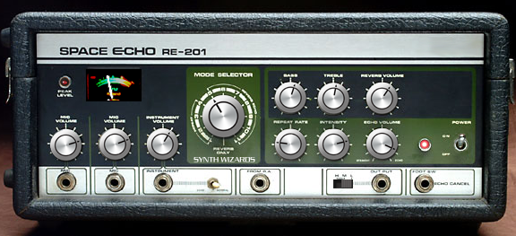
Eye had some extra time today so reworked this as test with my old projects. My goto VST effects unit has been SynthWizards Re501 so dug back into this project since there are some features rarely ever use on the 501. Rebuilding my 201 for true stereo versus mono insert saves me some CPU considering not using SOS(Sound On Sound) function most of the time. The method Eye used for the spring reverb on this VST sounds way better In My Opinion… especially on vintage analog drum machines. SynthWizards RE201 Stereo is another one of thee Wizards “Secret Weapons” . You can really hear my old obsession with repairing/modifying tape echo/delay machines in this VST. Plus, there is always that special satisfaction when your getting awesome sounds using something you have spent time designing/creating that can’t be replicated or emulated.

This module is a “tribute” module, based on the awesome Steiner-Parker Synthacon VCF. Those who know me will know I’m not a big VCF fan. Nonetheless, this VCF really appeals to me. This time I have added an optional input mixer, as well as extending the range of the filter. Extra adjustments are also possible.
How to use this module:
Connect the CV input to a voltage source such as a keyboard, envelope generator or sequencer. Connect the output to a VCA or amplifier. Feed the signal to be filtered into the high-pass, band-pass or low-pass input.
Unlike the original, this version allows signals to be fed into all inputs simultaneously. If the same signal is used in all inputs, the result is reminiscent of a phaser. The real fun starts when you feed different signals into each input, then you get a frequency based “interpolating scanner”, where panning between different sound sources is possible, though also subject to the frequency at which they are running. I have never heard an effect like it before.
Each of the filter type inputs has its own level control. The ALL input is also affected by these level pots as it mixed with the individual inputs prior to the level controls.
If using only a single input, it may be better to feed the signal into the ALL input, and adjust the level pots to select LP, BP or HP, rather than changing the patch cord between the specific input jacks.
A little on how it works:
The circuit uses a standard, non-inverting amplifier configuration. The three modes (HP, BP, LP) are obtained by injecting the signal into three different points of the circuit. An increase in the gain of the amplifier increases the filter’s Q. The Q remains almost constant as the filter is swept across the audio spectrum.
In the circuit, diode strings are used as voltage controlled resistors. The differential-amplifier transistors apply the bias voltage to the parallel diode string RC networks in opposing phase. The opposing phases cancel the control voltage so that none appears at the output.
The final pair of transistors form a non-inverting amplifier. The variable resistor adjusts the gain of this amplifier, and thus its Q.
The final stage is a simple gain stage, as I found the original was too quiet for my needs. The feedback resistor (RG) can be increased for more output level, or reduced for less. Start with 100k.
(Based on an article by Nyle Steiner from Electronic Design 25, Dec 6th, 1974.)

Before you start assembly, check the board for etching faults. Look for any shorts between tracks, or open circuits due to over etching. Take this opportunity to sand the edges of the board if needed, removing any splinters or rough edges.
When you are happy with the printed circuit board, construction can proceed as normal, starting with the resistors first, followed by the IC socket if used, then moving onto the taller components.
Take particular care with the orientation of the polarized components, the electrolytics and IC and transistors.
When inserting the IC in its socket, if used, take care not to accidentally bend any of the pins under the chip. Also, make sure the notch on the chip is aligned with the notch marked on the PCB overlay.
There are two ways this module cab be assembled – with the input level pots and ALL input, and without. The first way uses all four PCBs, the second only two, and a few lengths of tinned copper wire.
The EUR35D board is designed to connect all three main PCBs, eliminating wiring. 90 degree pin headers are used to achieve this. See the photos. It is designed to space the pots and jacks at one inch centers on the panel. Note that in this configuration, the bottom jack of the input board is the ALL input and the CV input is below the level pots.
If omitting the EUR35C level pot board, the EUR35D must also be omitted. Instead, tinned copper wire is run between the following pads on the input jack board (EUR35B) and the main board (EUR35A): 0V, HP, BP, LP, CV. Note that in this configuration, the bottom jack of the input board is the CV input.
Small square pads on the rear of the circuit boards are for 100n 1206 SMT decoupling capacitors. Positions are marked in dark grey on the overlay above.
On the overlay above two resistors are marked in different colors. If you find you have insufficient resonance, replace the 2k2 marked in red with a trimpot in the range of 2k to 4k7. You should now be able to adjust the resonance to a suitable level. This may be needed to compensate for variations in transistor gains.
The resistor marked in blue can be replaced with a trimpot in the range of 2k to 4k7, its purpose being to set the minimum resonance resistance. It’s function is not dissimilar to the trimmer mentioned above. It is most likely to be used to offset the range of the pot. It is also best if the trimmer is never adjusted to zero. Perhaps a 470ohm could be wired inline. It is unlikely this modification will be needed.
On the boards with pots, the jacks will need to be mounted on short lengths of tinned copper wire. Either solder tag or PCB mount Cliff jacks can be used. (CL 1366?)
IMPORTANT! Further builds have discovered a problem when running this design on 12 volts. If you wish to run on 12 volts and find the module hard or impossible to set up due to uncontrollable resonance, short out every third diode in the diode divider chain. It will still work on 15 volts with these diodes shorted out.
A quick and dirty guide to trimming:
If need be, adjust the resonance pot and resonance trimmer until it stops squeaking. Feed a LFO square wave in to the CV with no signal at the inputs. Adjust the CV span to get some response. Adjust CV reject for minimum thump. Turn resonance up. Adjust the resonance trim so that the screech can be controlled. It will depend on the initial frequency pot setting somewhat, so you will need to tweak it so you have acceptable resonance at the low frequencies, while not being uncontrollable or stoppable at the top of the frequency range. CV span – adjust it so you get more or less one octave per volt. Don’t waste too much time here. There is no way it will be either accurate or thermally stable. Be aware that unstable and “nasty” resonances are a feature of the sallen-key filter.
 Close up of one of the 90 degree headers.
 Front view of the assembly. Note the zigzag wire links to the floating jacks, and the orientation of the 90 degree headers used to join the boards together.
 Identification of the jacks and pots. The grid is 1 inch.
|
|||||||||||||||||||||||||||||||||||||||||||||||||||||||||||||||||||||||||||||||||||||
Parts list
This is a guide only. Parts needed will vary with individual constructor’s needs.
If anyone is interested in buying these boards, please check the PCBs for Sale page to see if I have any in stock.
Can’t find the parts? See the parts FAQ to see if I’ve already answered the question. Also see the CGS Synth discussion group.
|
 |
 |
Schematic |
 |
|
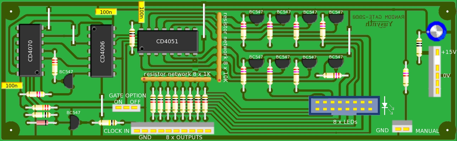
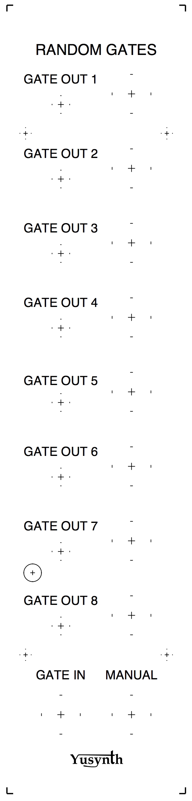
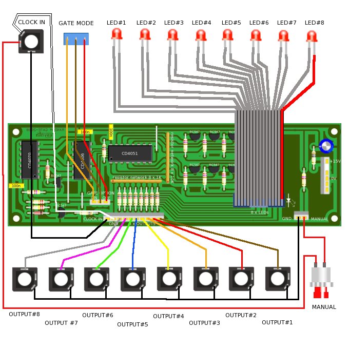
Basically, the circuit contains three main parts : the clock input built with Q1, the pseudo random sequence generator built with Q2, U1 and U3; and the addressing and output stages built with U2 and Q3 to Q10.
The core of the module is the pseudo-random sequence generator, it is in fact a classical circuit (Elektor) uses to generate digital noise. The CD4006 is an eigtheen stage shift register whose some of its outputs are fedback to its input through XOR gates (CD4070). Q2 inverses one of the output before applying to the XOR gate input in order to avoid an all zero status that would block the generator. The random generator is clocked by an external signal which is buffered by Q1, then a XOR gate of U3d is used to straighten the edges of the clock pulses : this was necessary to make this circuit work with some brands of the 4006 (HEF4006,MC14006) which required more stringent pulse conditions. Three outputs of the CD4006 are connected to the binary addressing pins (A,B,C) of the CD4051 (8 voice analogue multiplexer). The common pin of the CD4051 is connected to the positive rail through a 1K resistor, and all the outputs are connected to an output buffer stage. The GATE MODE switch controls the INHIBIT pin of the CD4051, in the OFF mode the INHIBIT pin is connected to the ground and the active output of the CD4051 remains active. In the ON mode the clock signal is routed to the INHIBIT pin and gates the active output.NOTE : after powering up, the module needs at least ten clock cycles before it gets into the expected behaviour. |
|
|
Printed Circuit Board and Component Layout |
|||
IMPORTANT NOTE : Don’t forget the five straps. Also because some tracks are quite thin and located very close to each others, check thoroughly the PCB tracks with a looking glass in order to detect the possible copper micro-bridges (ill-etching) and track micro-cuts. |
| , |
|
List of parts and building instructions |
|||||||||||||||||||||||||||||||||||||||||||||||||||||||||||||||||||||
|
|||||||||||||||||||||||||||||||||||||||||||||||||||||||||||||||||||||
| Wiring | |||||||||||||||||||||||||||||||||||||||||||||||||||||||||||||||||||||
|
|
|
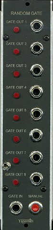
| Front plate | ||
|
|
|
Trimming |
| This circuit requires no trimming. It must work when powered on. NOTE : after powering up, the module needs at least ten clock cycles before it gets into the expected behaviour. |
|
|
Modifications of the old PCB |
| NOTE : these modifications are only for those who built the circuit with the old PCB
Remove the long strap between the collector of Q1 (lowest transistor on the layout) and pin 3 of U1 (4006).
With an sharp knife cut the short track from pad 13 of U3 (4070), connect a short isolated wire between pad 11 of U3 and pad 3 of U1, connect a short isolated wire between pad 13 of U3 and the collector of Q1. |
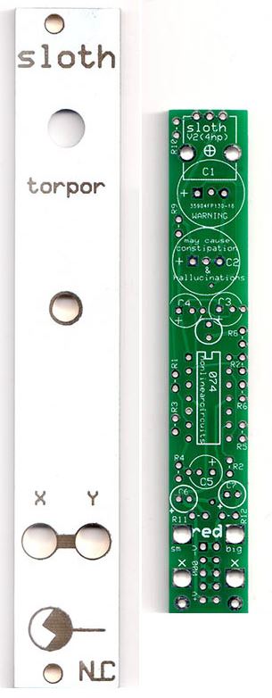
This is a very simple to build chaos module that can be built in 2 ways: slow or VERY slow. Slow means 1 cycle every 15 seconds, VERY slow is 1 cycle every 15 minutes. It can take up to an hour for any change to be apparent when tweaking the pot. This module is ideal for ambience and extremely patient synth users. I developed it as I like to have my synths running whilst soldering away in the workshop and I like slow never-repeating changes to the patches.
The PCB is 16 x 95 mm, suitable for 4HP eurorack panels (panels will be available soon)
PCBs are available now (13/9/2014) for $8 each.
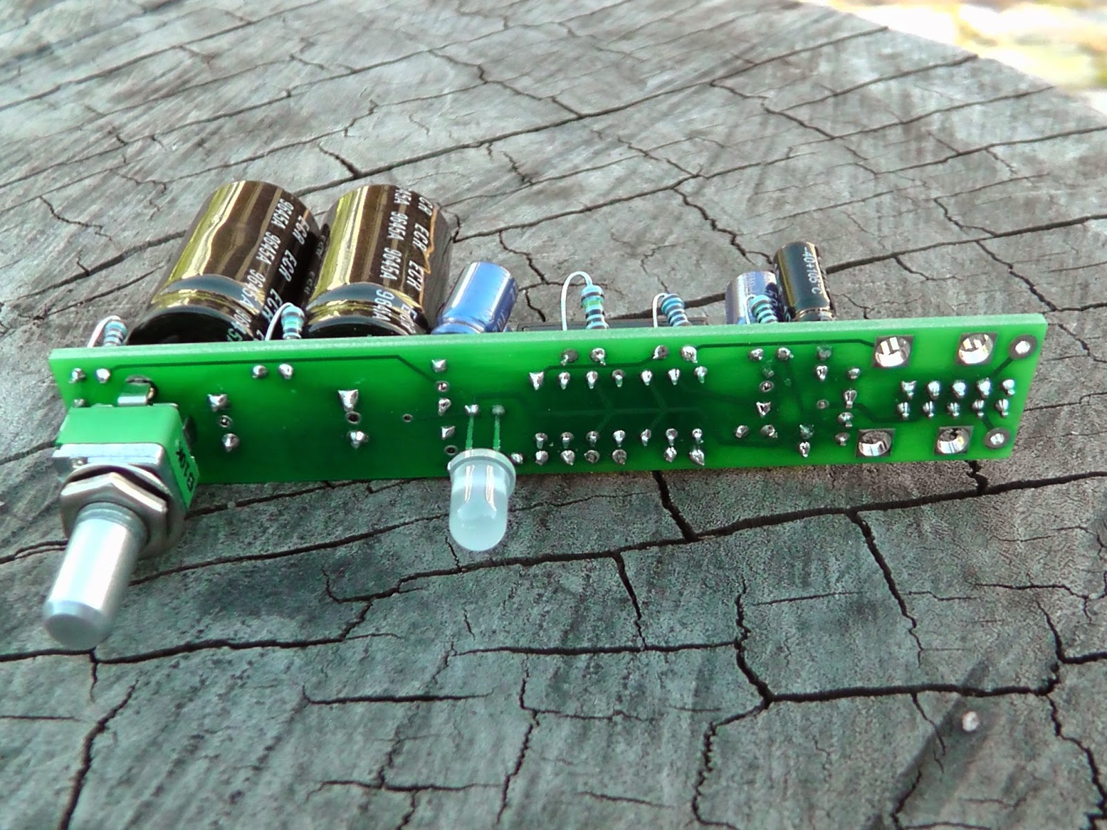
Shipping is $5 per orderThe super slow version shown below has two 1000uF caps.


Copyright � 1971 Poptronix, Inc.; used by permission.
Build the PSYCH-TONE Melody Synthesizer
By Don Lancaster
Ultimate Decimal Counter
By Daniel Meyer
The PSYCH-TONE in the photos above sold on eBay for $360 in September 2005.
Here is a note I got from someone that shall remain nameless.
Thank you, sir. Your SWTPC site has been a time machine for me (and others, I’m sure).
Going over your SWTPC catalogs, it must have been 1971 when I saw the Psych-Tone – first in a Popular Electronics article and then in their catalog. I had to have it. I could handle a soldering iron – I had to build it! I saved (and begged my father) and ordered the kit. I must have fried a number of components because the thing never produced anything more than static (thank the Gawds it didn’t start smoking). I’m fairly sure it got lost (or trashed) in the course of moving.
Each page is a 150 dpi jpg image.
300 dpi tiff files are available.