Even if you don’t know an ohm from a volt, Craig Anderton’s revised and expanded book shows you how to build 27 accessories that enhance your sound and broaden your musical horizons. If you’re an old hand at musical electronics, you’ll really appreciate that all of the processors, from tube sound fuzz to phase shifter are compatible and work together without creating noise, signal loss, bandwidth compression or any of the other problems common to interconnecting effects from different manufacturers. There’s even a complete chapter on how to modify and combine effects to produce your own custom pedal board. Low cost project kits available from PAiA help make even your first exposure to electronics a pleasant, hassle-free experience and thanks to CD bound into the book, you know just how the device will sound before you even start.

http://www.adjutojunior.com.br/eletronica_basica/ELECTRONIC_PROJECTS_FOR_MUSICIANS_by_Craig_Anderton.pdf

How the Enlightenment Ends

Philosophically, intellectually—in every way—human society is unprepared for the rise of artificial intelligence.

Henry A. Kissinger
June 2018

https://www.theatlantic.com/magazine/archive/2018/06/henry-kissinger-a i-could-mean-the-end-of-human-history/559124/

http://www.glensstuff.com/

http://www.glensstuff.com/hyperrossler/hyperrossler.htm

http://www.glensstuff.com/sprottsystems/sprottsystems.htm

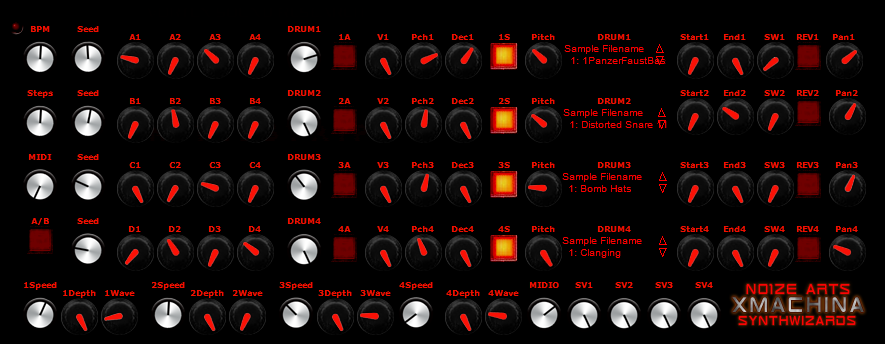
XMACHINA is a Probability Auto Generative Drum Machine Engine with 4 BPM sync LFOs autopanning each sound while modulating “seed” factors that plays drum samples plus has built in CR78/MFB502 type Drum Synth that also transmits 4 channels of generated MIDI patterns for driving hardware at same time from the “Probabilty” Engine… XMACHINA also directly writes multichannel MIDI data compositions into DAW

xn+1= 1 – axn2 + bxn,
(a and b are parameters)

Michel Henon, an astronomer at the observatory in Nice, France, was born in Paris in 1931. Curious about the degradation of celestial orbits, he began to model the orbits of stars around the centers of their galaxies.
Henon considered gravitational centers as a three dimensional object (as opposed to a point in space) and carefully studied the orbits of the stars. To simplify the task of trying to track a three dimensional orbit, he considered, instead, the intersection of a plane with these orbits. Initially, the intersection points appeared to be completely random in their location, moving from one edge of the plane to the next. However, after a few dozen points were plotted, a closed, egg-shaped curve began to appear. This mapping was, apparently, the cross section of a torus (i.e., a doughnut).
Henon (along with one of his graduate students) continued to study this mapping and continued plotting the points for a system with increased energy levels. Once the newer mappings were made, though, the continuous curve began fading and random points began to appear proportionally to the energy. Over the years, Henon tried many ways to predict the upcoming points of his high-energy graph until finally, he decided to abandon classical methods and use difference equations.
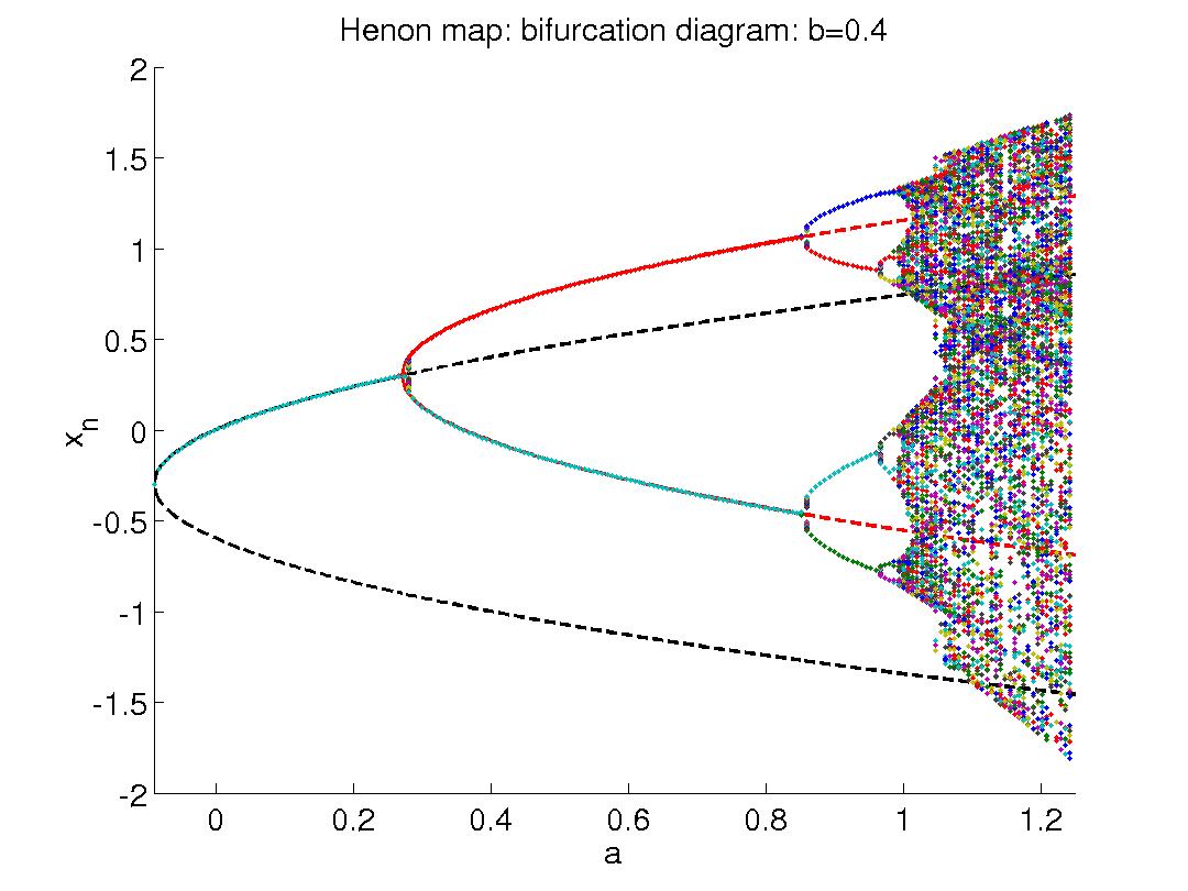
Applying a formula to force the data into the shape of a crescent moon, Henon found some interesting results. The formula was fairly simple. Take the old y and multiply it by 0.3 (b). Then subtract 1.4 (a) times the old x squared. Finally add one to the whole equation. This yields this system:

xnew= y – 1.4×2 + 1
ynew= 0.3x

Although, at first, it seems like an ordinary curve, closer inspection reveals distinct curves, one thicker than the other. If we magnify the picture, we see that each of these curves is also made up of two similar curves. This happens for every possible magnification of the curve.

In astronomy, Michel Hénon was a leading figure in the field of stellar dynamics, galactic dynamics, and the evolution of the rings of Saturn. In mathematics, he is known for the so-called Hénon maps and attractor, which is one of the most studied chaotic systems.
In the late 1960s and early 70s, he worked on the star clusters and by using Monte Carlo methods, he developed numerical techniques to follow the dynamics of globular clusters. His probabilistic method proved to be much faster than usual N-body methods.
He published a two volume book on restricted three-body problem.

He died on April 2013 in Nice.
http://adsabs.harvard.edu/cgi-bin/nph-a … &version=1
https://arxiv.org/pdf/1411.4930
https://www.youtube.com/playlist?list=P … 6-akNgLG7-_

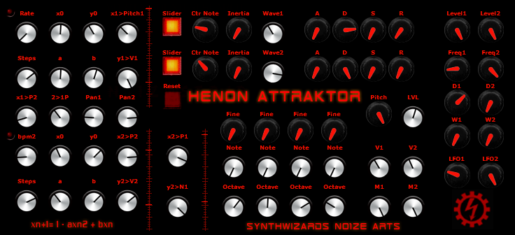
Dual Midi Channel Generative Sequencer
xn+1= 1 – axn2 + bxn
2 “iterations” of formula cross modulating
plus 2x LFO modulating params
generating evolving sequences
includes built in sound engine
works with “Hardware”
“Esoteric” Henon MIDI Sequencer….

In 1963 Edward Lorenz published his famous set of coupled nonlinear
first-order ordinary differential equations; they are relatively simple,
but the resulting behavior is wonderfully complex. The equations are:

dx/dt = s(y-x)
dy/dt = rx-y-xz
dz/dt = xy – bz

with suggested parameters s=10, r=28, and b=8/3. The solution executes
a trajectory, plotted in three dimensions, that winds around and around,
neither predictable nor random, occupying a region known as its attractor.
With lots of computing power you can approximate the equations numerically,
and many handsome plots can be found on the web. However, it’s rather
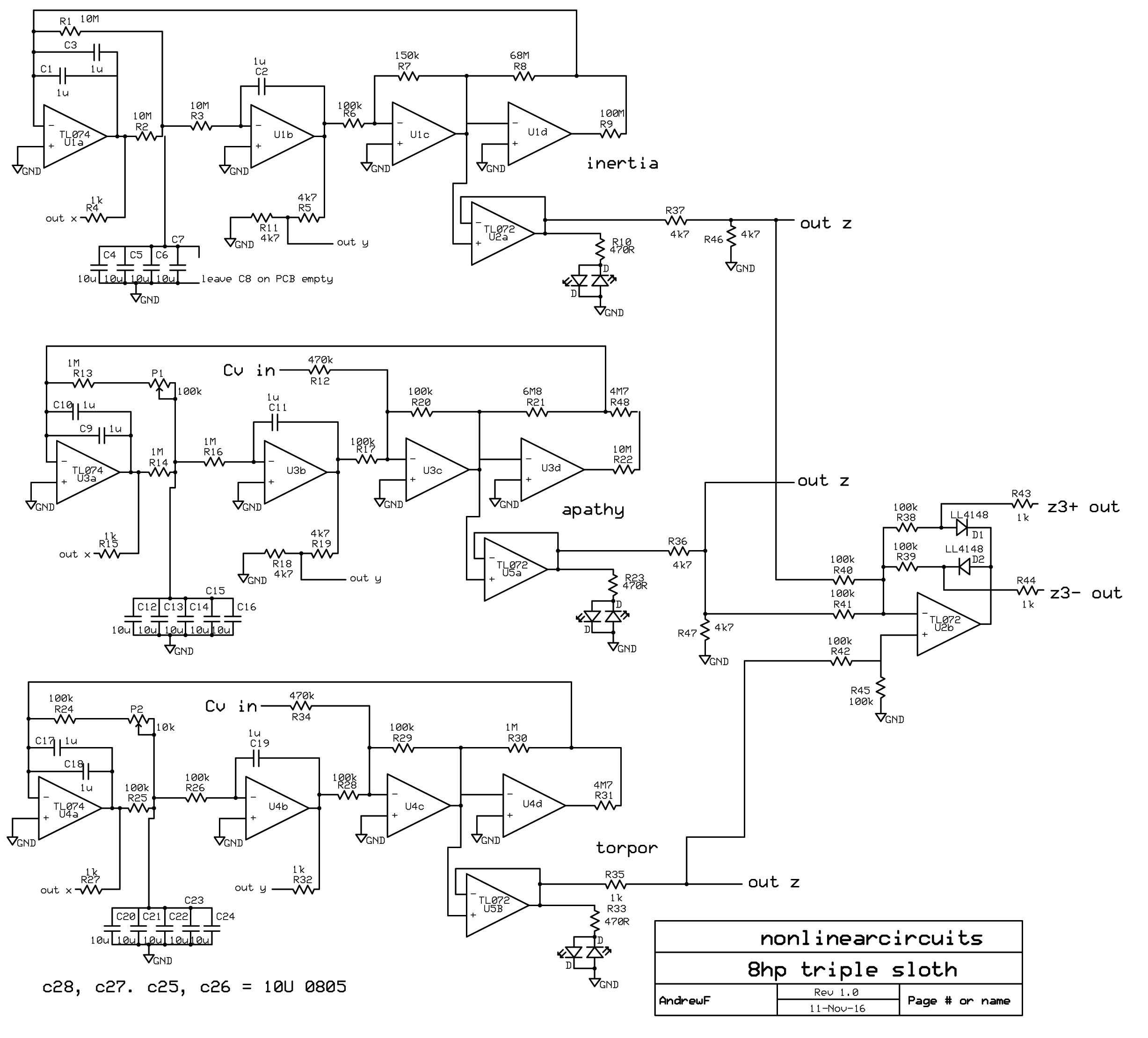
easy to implement these equations in an analog electronic circuit, with
just 3 op-amps (each does both an integration and a sum) and two analog
multipliers (to form the products xy and xz).

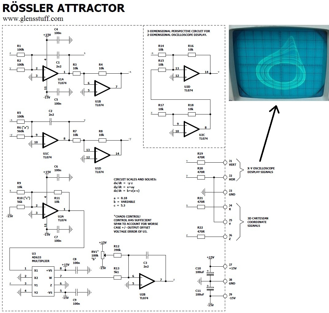
The Circuit

Here’s the circuit:

It’s not hard to understand: the op-amps are wired as integrators, with
the various terms that make up each derivative summed at the inputs. The
resistor values are scaled to 1 megohm, thus for example R3 weights the
variable x with a factor of 28 (1M/35.7k); this is combined with -y and
-xz, each with unit weight. (note: the equations on the diagram are
normalized to 0.1V, hence the multiplier scale factor of 100.)

The Output

The circuit just sits there and produces three voltages x(t), y(t), and z(t);
if you hook x and z into a `scope, you get a pattern like this…

…the characteristic “owl’s face” of the Lorenz attractor. The curve
plays out in time, sometimes appearing to hesitate as it scales the
boundary and decides which basin to drop back into. The value of C, the
three integrator capacitors, sets the time scale: at 0.47uF it does a
leisurely wander; at 0.1uF it winds around like someone on a mission; and
at 0.002uF it is fiercely busy solving its equations and delighting its
audience.
http://www.malinc.se/m/Lorenz.php
http://physics.ucsc.edu/~drip/programs/lorenz/
Now whatever could that be used for in “NOISE”?

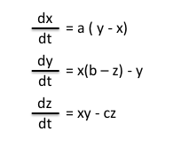
There are three Lorenz equations that comprise the Lorenz Attractor, each of which can be though of as the x, y, or z component of a given three dimensional location in space:

Each of these equations can be read as the ‘change in x,y, or z with respect to time’. Thus, each equation is used to calculate how much a given point is changed relative to the previous point, the change dependent upon the elapsed time.

The values a, b, c in the Lorenz equations are constants (for the Lorenz Attractor, a = 10, b = 28, and c = 8/3). These constants, as well as the above equations, can be altered to generate different results. For instance, a value of a = 1 results in a spiral with a single attractor (converging on this attractor), or a value of c = 20 results in a similar pattern given by c = 28, but with more compact orbits. Alternatively, other mathematical equations result in other types of attractors, such as the Henon Map or the Rossler Attractor.

Eye needed super lightweight basic 2xVCO Noise RingMod BPM sync LFO & ADSR VST so slapped together N01ZESTRIP. This is a basic reference synth sound source when creating elaborate  MIDI files with KAOTIKA… when have all the MIDI recorded it is far easier adding hardware… funny thing is this simple low CPU usage VST N01ZESTRIP sounds surprisingly good 😛 Made specifically for use with KAOTIKA